Ugh. Shoulda been literally anyone else in the final four. I’m NOT mad.

Unfortunately, the incredibly fun and chaotic 2023 Men’s College Basketball tournament had a real stinker of an ending, as UConn went berserk en route to their fifth championship and third since 2010. And not only did they beat everyone, they absolutely demolished the hell out of everyone, notching double-digit victories in all six games of their run. Disgusting.

But how does this rank among the all-time great tournament runs? Were they more dominant than the great Duke and Kentucky teams of old? I decided to use the awe-inspiring, earth-shattering power of the R statistical programming language to find out. Let’s rock and roll.

Finding some data

Let’s start by finding some data. In order to figure this out, we’ll need the scores of every single NCAA tournament game played in the timespan we’re interested in. For our purposes, I’ll be looking for data from the year the field expanded to 64 teams (1985) onward. I looked around on my favorite internet search engine for a bit, and found this website that seems to have all the data I need. Nice!

Now we just need to scrape it real quick so we can use it in R. We’ll get to work with the {rvest} package, my go-to when it comes to static web scraping.

library(dplyr)
library(lubridate)
library(janitor)
library(rvest)

# Start by grabbing the html from our website
page <- rvest::read_html("http://www.hoopstournament.net/DynamicDrilldown.php")

# html_table() will pull the info out of all the tables on the page. Easy!
content <- page |>
  html_table()

# The first and second tables are just for structural purposes on the site,
# so we're interested in the third one, where the actual data is.
ds <- content[3][[1]] |> 
  clean_names() |>
  # Let's clean it up and add some useful variables
  mutate(
    date = mdy(date),
    year = year(date),
    team_year = paste0(team, " (", year, ")"),
    margin = score - opp_score
  ) |>
  # Lastly, filter out the years we don't care about
  filter(year >= 1985)

head(ds)

## # A tibble: 6 × 15
##   date        seed team             seed_2 opponent  w_l   score opp_score round
##   <date>     <int> <chr>             <int> <chr>     <chr> <int>     <int> <chr>
## 1 2023-04-03     4 Connecticut           5 San Dieg… W        76        59 Nati…
## 2 2023-04-03     5 San Diego State       4 Connecti… L        59        76 Nati…
## 3 2023-04-01     4 Connecticut           5 Miami, F… W        72        59 Nati…
## 4 2023-04-01     9 Florida Atlantic      5 San Dieg… L        71        72 Nati…
## 5 2023-04-01     5 Miami, Florida        4 Connecti… L        59        72 Nati…
## 6 2023-04-01     5 San Diego State       9 Florida … W        72        71 Nati…
## # ℹ 6 more variables: location_city <chr>, location_state <chr>,
## #   box_score <chr>, year <dbl>, team_year <chr>, margin <int>

Looks like we got it! This also inclues the play-in / first four games for the years since those were added. Next, we’ll need to summarize by team_year to see which team had the biggest cumulative / average victory margin. Simple!

# First we need to figure out which team_year values ended up winning it all.
champs <- ds |>
  filter(round == "National Championship" & w_l == "W")

tourney_runs <- ds |>
  # champs only!
  filter(team_year %in% champs$team_year) |> 
  group_by(team_year) |>
  summarize(
    team = unique(team),
    seed = unique(seed),
    cum_margin = sum(margin),
    avg_margin = mean(margin),
    n_games = n(),
    list_margins = paste(margin, collapse = ", ")
  ) |>
  arrange(desc(cum_margin))

# Let's look at the top 10:
library(kableExtra)

tourney_runs |>
  select(-team) |>
  slice_max(order_by = cum_margin, n = 10) |>
  kable()

team_year	seed	cum_margin	avg_margin	n_games	list_margins
Kentucky (1996)	1	129	21.50000	6	9, 7, 20, 31, 24, 38
Villanova (2016)	2	124	20.66667	6	3, 44, 5, 23, 19, 30
North Carolina (2009)	1	121	20.16667	6	17, 14, 12, 21, 14, 43
Connecticut (2023)	4	120	20.00000	6	17, 13, 28, 23, 15, 24
Nevada-Las Vegas (1990)	1	112	18.66667	6	30, 9, 30, 2, 11, 30
Villanova (2018)	1	106	17.66667	6	17, 16, 12, 12, 23, 26
Duke (2001)	1	100	16.66667	6	10, 11, 10, 13, 13, 43
Louisville (2013)	1	97	16.16667	6	6, 4, 22, 8, 26, 31
Florida (2006)	3	96	16.00000	6	16, 15, 13, 4, 22, 26
North Carolina (1993)	1	94	15.66667	6	6, 10, 7, 6, 45, 20

Well look who’s sitting there are #4 all time! It’s 2023 UConn, who beat their opponents by an average of 20 points! Also notice their #4 seed – everyone else in the immediate vicinity is either a #1 or a #2. ’96 Kentucky is #1, and interestingly, Duke doesn’t show up until #7. Coach K = fraud confirmed. Also just want to give a quick “I hate you” to 2018 Nova. You know what you did.

Let’s make a few fun graphs just to really put this in context. First, I’m going to grab some team color / logo / etc. data from {hoopR} and join it onto our dataset for ~aesthetic~ purposes.

library(hoopR)

ds_teams <- espn_mbb_teams() |>
  # The team names don't quite match up, so I'm just gonna fix em manually
  mutate(team = case_when(
    team == "UConn" ~ "Connecticut",
    team == "LSU" ~ "Louisiana State",
    team == "UMass" ~ "Massachusetts",
    team == "Nevada" ~ "Nevada-Las Vegas",
    team == "NC State" ~ "North Carolina State",
    team == "VCU" ~ "Virginia Commonwealth",
    team == "Miami" ~ "Miami, Florida",
    TRUE ~ team
  ))

tourney_runs <- left_join(tourney_runs, ds_teams, by = "team")

Next, we’ll plot all the tournament runs by cumulative victory margin. I’m also going to go a little nuts with the annotations because I also want to see how many standard deviations above / below average each run was. There’s probably a more elegant way to add these annotations; maybe a package or something? Maybe I should make a package if one doesn’t exist.

library(ggplot2)
library(ggimage)
library(ggthemes)

tourney_runs |>
  ggplot(aes(x = reorder(team_year, -cum_margin),
             y = cum_margin,
             fill = team)) +
  # St. Deviations
  annotate(geom = "rect",
           xmin = -Inf, xmax = Inf,
           ymin = mean(tourney_runs$cum_margin) + 0.5, 
           ymax = mean(tourney_runs$cum_margin) + 1 * sd(tourney_runs$cum_margin) - 0.5,
           alpha = 0.2) +
  annotate(geom = "rect",
           xmin = -Inf, xmax = Inf,
           ymin = mean(tourney_runs$cum_margin) + 1 * sd(tourney_runs$cum_margin) + 0.5,
           ymax = mean(tourney_runs$cum_margin) + 2 * sd(tourney_runs$cum_margin) - 0.5,
           alpha = 0.4) +
  annotate(geom = "rect",
           xmin = -Inf, xmax = Inf,
           ymin = mean(tourney_runs$cum_margin) - 0.5, 
           ymax = mean(tourney_runs$cum_margin) - 1 * sd(tourney_runs$cum_margin) + 0.5,
           alpha = 0.2) +
  annotate(geom = "rect",
           xmin = -Inf, xmax = Inf,
           ymin = mean(tourney_runs$cum_margin) - 1 * sd(tourney_runs$cum_margin) - 0.5,
           ymax = mean(tourney_runs$cum_margin) - 2 * sd(tourney_runs$cum_margin) + 0.5,
           alpha = 0.4) +
  annotate(geom = "rect",
           xmin = -Inf, xmax = Inf,
           ymin = mean(tourney_runs$cum_margin) - 2 * sd(tourney_runs$cum_margin) - 0.5,
           ymax = 0, 
           alpha = 0.6) +
  # Columns
  geom_col() +
  annotate(geom = "text",
           color = "#5A5A5A",
           label = "AVERAGE",
           size = 5,
           x = 35,
           y = mean(tourney_runs$cum_margin)) +
  # Std. dv labels
  annotate(geom = "text",
           label = "+1 std. deviation",
           size = 5,
           color = "white",
           x = 35,
           y = mean(tourney_runs$cum_margin) + 1 * sd(tourney_runs$cum_margin) - 3) +
  annotate(geom = "text",
           label = "+2 std. deviations",
           size = 5,
           color = "white",
           x = 35,
           y = mean(tourney_runs$cum_margin) + 2 * sd(tourney_runs$cum_margin) - 3) +
  annotate(geom = "text",
           label = "-1 std. deviation",
           size = 5,
           color = "white",
           x = 35,
           y = mean(tourney_runs$cum_margin) - 1 * sd(tourney_runs$cum_margin) + 3) +
  annotate(geom = "text",
           label = "-2 std. deviations",
           size = 5,
           color = "white",
           x = 35,
           y = mean(tourney_runs$cum_margin) - 2 * sd(tourney_runs$cum_margin) + 3) +
  # Arrows
  annotate(geom = "segment",
           x = 12, xend = 4.5,
           y = 128, yend = 120,
           arrow = arrow(type = "closed"),
           size = 0.5
  ) +
  annotate(geom = "label",
           x = 12, y = 130,
           label = "UConn (2023)") +
  # Other styling
  scale_fill_manual(values = paste0("#", tourney_runs$color),
                    breaks = tourney_runs$team) +
  labs(
    title = "Most Dominant NCAA Tournament Championship Runs",
    subtitle = "by cumulative margin of victory, all tournaments since 1985",
    x = "Team / Year",
    y = "Cumulative Margin of Victory",
    caption = "Data from http://www.hoopstournament.net/"
  ) +
  guides(fill = "none") +
  theme_fivethirtyeight() +
  theme(
    axis.text.x = element_text(angle = 45, hjust = 1)
  )

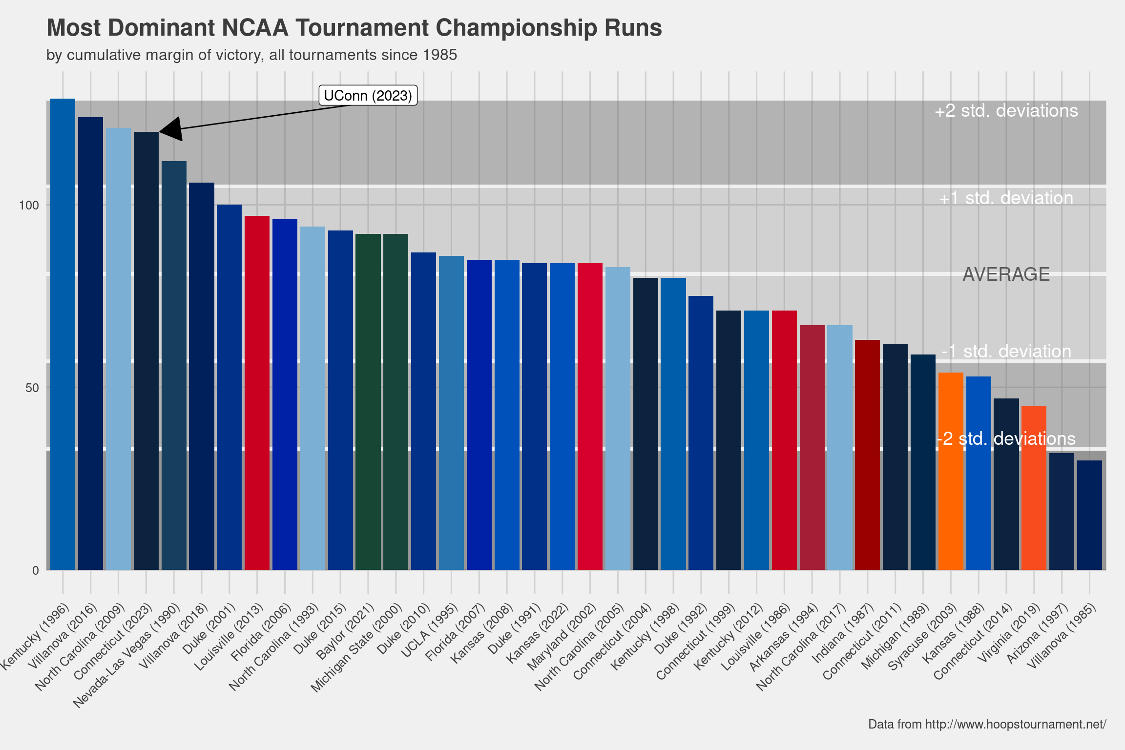
Pretty impressive stuff! They certainly benefited from the chaos quite a bit (just like KU did last year, actually), and only ended up playing one team that finished in the Kenpom top 10 (#8 Gonzaga). They didn’t have to play UCLA, KU, Texas, Alabama, Purdue, Houston, Marquette, or Arizona, which was practically my entire (plus UConn themselves) pre-tourney list of possible contenders.

But you can only beat who you play, and they did that better than almost anyone else ever has. If any UConn fan stumbles across this, congrats! 😒